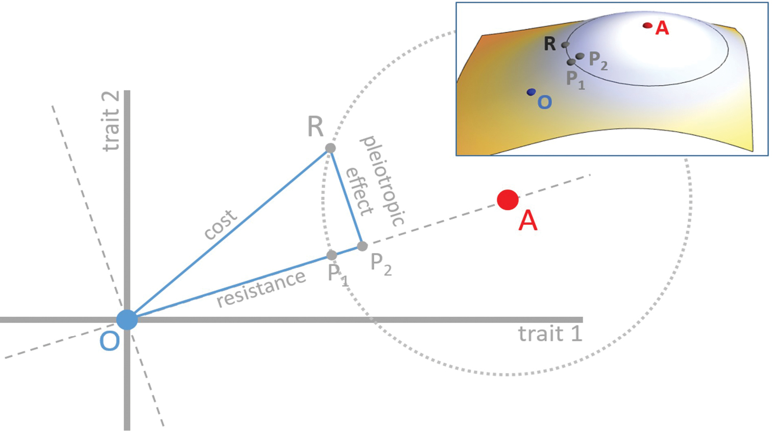
Graph of treated and non-treated environments, with distinct phenotypic requirements (phenotypic optima A and O, respectively) in a two-trait space. Assuming a wild-type positioned in O, the resistance mutation R brings the phenotype closer to A. Relative to the wild type, R is therefore a beneficial mutation in the treated environment. Its cost is usually defined as its fitness in the non-treated environment relative to the wild type, which depends on the distance between R and O on the figure. Note that the cost (and all fitness measures on this figure, and similar figure below) depends on Euclidian distances in phenotypic space, and a mapping function converting this distance to fitness (i.e. the cost is not distance OR, but a monotonic function of this distance). The mapping is left implicit on the figure, but can be thought as a third orthogonal axis representing fitness for each trait 1 – trait 2 combination, which defines a “fitness landscape”. The coloured inset figure represents such a fitness mapping in 3D. Fitness values, when projected on the phenotypic space correspond to isofitness curves (like altitude on a geographic map is indicated by contour lines). For instance all phenotypes on the light grey circles have the same fitness than mutation R in the treated environment (optimum A). The direction of the two optima (OA axis) defines a phenotypic trait of ‘resistance’. Variation of trait(s) orthogonal to this axis may be defined as pleiotropic effects. Point P1 on OA axis is such that AR = AP1. It represents the phenotypic point that would confer the same fitness in the treated environment compared to the mutation R, but that would only alter the phenotype in the exact direction of the optimum A. Point P2 is the orthogonal projection of R on OA axis. It represents the phenotypic point that would be reached if all the pleiotropic effects of the mutation R were compensated (e.g. by subsequent compensatory mutations).